What is LoRa and when should it be used?

With the recent advancements in LLMs, the size of models continues to grow, and fine-tuning models is becoming increasingly expensive. The rise of this issue led to an increased interest in parameter-efficient fine-tuning (PEFT) techniques. With over 15,000 citations ¹, Low-Rank Adaptation of Large Language Models (LoRa) is one of the world’s most popular PEFT techniques.

LoRa is a great technique for minimizing memory requirements when fine-tuning LLMs or other large neural networks and cutting down on storage costs when deploying multiple adaptations of the same model while suffering negligible performance degradation.

In this article, we will first understand the workings of LoRa. Then, we’re going to support the argument mentioned earlier and see how LoRa offers efficiency.

1 How does LoRa work?

Before we introduce LoRa, let’s consider how classic fine-tuning works. Let’s say you have a pre-trained weight matrix \(W_0 \in \mathbb{R}^{m \times n}\). In classical fine-tuning, the task is to find a new weight matrix \({\displaystyle \Delta }W \in \mathbb{R}^{m \times n}\) such that the layer output \(y = W_0x + {\displaystyle \Delta }Wx\) minimizes the cost function of the new training dataset.

Note that in this method, we have \(m \times n\) learnable parameters corresponding to each entry in the \({\displaystyle \Delta }W\) matrix as each value is computed independently of the others.

LoRa uses the same general formula but computes \({\displaystyle \Delta }W\) differently. LoRa defines the \({\displaystyle \Delta }W\) by decomposing it in the following manner.

\[{\displaystyle \Delta }W = BA\]

where \(B \in \mathbb{R}^{m \times r}\), \(A \in \mathbb{R}^{r \times n}\), and \(r << min(m, n)\). Note that the product of \(B\) and \(A\) has the same dimension as the original \({\displaystyle \Delta }W\) matrix; hence, this decomposition is valid and we can plug it into the equation defining the new output.

Now, the number of trainable parameters is \(r(m + n)\). Since \(r\) is much smaller than both \(m\) and \(n\), the number of trainable parameters in LoRa is much less than that of classical fine-tuning.

2 Memory Efficiency

The first thing I want to highlight about LoRa is its memory efficiency. According to (Hu et al. 2021), LoRa reduces VRAM usage by up to two-thirds for large transformers trained by Adam provided we choose an appropriate value for \(r\).

During classical fine-tuning, we need to store the full optimizer state for all parameters in the model since they are all trainable. Since \(r\) is much smaller than the dimension of the original matrix, in LoRa the number of parameters to train is much smaller consuming less memory space.

With the continuous increase in LLM sizes, memory is becoming the bottleneck for fine-tuning LLM tasks. LoRa permits us to work with large models without spending large sums of money on huge VRAM GPUs.

A positive side-effect caused by the VRAM minimzation is the need of less GPU-hours. Since less memory is needed when LoRa is used, we can use a bigger batch size using the same GPU. THe increase in batch leads to a decrease in training time.

3 Storage Cost Cuts

When you use classical fine-tuning, all of the model’s weights are updated. So you end up with a huge number of new weights, equaling the size of the original model.

Suppose you’re fine-tuning a certain foundational model that contains 100 billion parameters for 10 different tasks using classical fine-tuning. After you finish training all the models, you want to deploy the 10 models. Let’s focus on the storage requirements imposed by such a scenario. Since you updated all weights while training each single model, you end up with \(10 \text{ billion} \times 10 = 1 \text{ trillion}\) new parameters. In general, when fine-tuning \(n\) models from the same foundational model, you end up having to store \(n\) times the size of the original model.

Therefore, classical fine-tuning inflicts enormous storage costs for organizations deploying multiple adaptations of a single model, which is a very common scenario for cloud-based machine learning services. It doesn’t scale well for multiple adaptaions.

LoRa comes to help also here. As seen in Section 1, the number of new parameters made by LoRa is much smaller than the number of parameters in the original model. When you deploy a model fine-tuned by LoRa, you need to store both the original model and all the new weights created. While this way requires slightly more space when deploying one model, it offers considerable savings when deploying multiple models because the huge foundational model is stored only once and only the few newly trained parameters are stored for each adaptaion.

Hu et al. (2021) demonstrate an example of the storage cost savings offered by LoRa. They state that fine-tuning GPT-3 175B using LoRa with \(r = 4\) and while adapting only the query and value projections reduces the checkpoint size roughly 10,000 times (350GB -> 35MB). So when storing a 100 model fine-tuned from GPT-3, the required storage is reduced from \(100 \times 350GB \approx 35TB\) to \(350GB + 100 \times 35MB \approx 354GB\). So around 99% of the costs are saved by LoRa.

4 Quality Conservation

As with any PEFT technique, there is always the fear that efficiency comes at the cost of quality. This isn’t the case here, however. LoRa manages to maintain the same or even improve the quality of the original model.

Actually, as the value \(r\) approaches \(min(m, n)\), LoRa becomes the same as classical fine-tuning. We can easily prove this.

Proof. Assume that \(min(m, n) = m\). If \(r = m\), then \(y\) becomes

\[y = W_0x + BAx\]

where \(B \in \mathbb{R}^{m \times m}\), \(A \in \mathbb{R}^{m \times n}\). By setting \(B\) to the identity matrix, LoRa becomes the same as classical fine-tuning as \(A\) converges to the same value as \(W\). The same argument can be applied if \(min(m, n) = n\) by flipping \(A\) and \(B\).

Hu et al. (2021) show experimental data supporting the high performance of LoRa-trained models.

Table 2 from Hu et al. (2021)

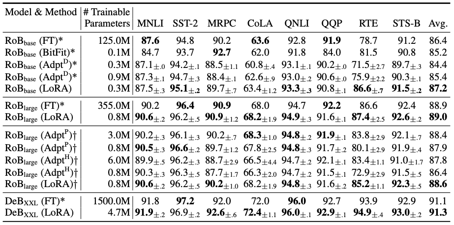
As you can see in the above figure, LoRa-tuned models perform very closely or even better than those using classical fine-tuning (marked FT in the figure).

5 Conclusion

In this article, we discussed the science behind LoRa and its advantages. We first began by uncovering how LoRa decomposes the \({\displaystyle \Delta }W\) matrix. Then, we showed that through updating a smaller number of parameters, LoRa stores less optimizer state and consumes less memory. By sharing the weights of the original model, LoRa offered considerable storage savings when deploying multiple variations of the same model. It does all that while maintaining the same quality of classical fine-tuning as demonstrated by experimental data and its convergence to classical fine-tuning.

Thanks for reading and I hope this article helped you learn a bit more about PEFT.

5.1 References

Hu, Edward J., Yelong Shen, Phillip Wallis, Zeyuan Allen-Zhu, Yuanzhi Li, Shean Wang, Lu Wang, and Weizhu Chen. 2021. “LoRA: Low-Rank Adaptation of Large Language Models.” https://arxiv.org/abs/2106.09685.

Footnotes

1. This number is based on Google Scholar on the date of publishing the article.